Top 5 Excel Formulas for Financial Modeling

Excel is an indispensable tool for financial modeling, and mastering its formulas can take your skills to the next level. Whether you're a beginner or an experienced modeler, understanding and applying the right formulas can save you time, reduce errors, and provide valuable insights into your financial data.

From calculating growth rates to performing scenario analysis, these formulas will help you build more accurate, efficient, and dynamic financial models.

Now, let's explore the five of the most important/most used formulas used when building a financial model in Excel.

1. SUM:

The Excel SUM function returns the sum of the values supplied. These values can be numbers, cell references, ranges, arrays, and constants in any combination.

The SUM function is essential to determine totals for line items in financial statements. For example, summing up all expenses into a single line item titled “COGS.”

Example:

=SUM(B2:B8) sums the cells in B2 through B8.

=SUM(B2:B4,B5:B8) would return the same value.

2. IF Statements: 

The IF function runs a logical test and returns one value for a TRUE result, and another value for a FALSE result. 

IF statements allow you to set conditions to trigger specific actions in the model. For example, if you want to model your hiring plan but anticipate different start dates for various employees, you can use IF statements to ensure that the cost related to that hire starts to occur once their intended start date is reached.

Example:

=IF(logical_test, [value_if_true], [value_if_false])

If you want to highlight expense buckets that were over or under budget, you can use an IF statement to easily identify each discrepancy.

=IF(B2>C2,”Over Budget”,”Met Budget”)

This means if the expense category is greater than the budgeted amount, the status should show as “Over Budget.” If the expense category is not greater than the budget, the output reads “Met Budget.”

To further enhance your financial model, more than one condition can be tested by nesting IF functions. The IF function can be combined with logical functions such as “=AND” and “=OR” to extend the logical test.

3. SUMIF:

Combine SUM and IF statements into a SUMIF function, which allows you to sum a range of values if certain conditions are met.

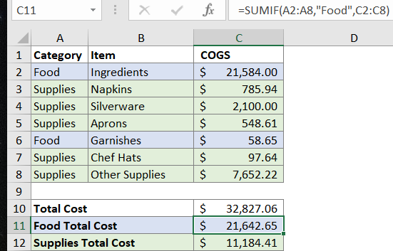
In the below example, you can determine the total cost of all items in the “Food” category and the total cost of all items in the “Supplies” category. 

To determine the cost of all food-related expenses, use the following formula:

=SUMIF(A2:A8,”Food”,C2:C8)

This tells Excel to search in the “Category” column A for the word “Food”, then sum the corresponding expenses in the “COGS” column for items in the Food category only.

4. IFAND: 

The AND function allows logical tests for multiple conditions to be met.

When coupled with the IF function, the AND function can be used as the logical test inside the IF function to avoid extra nested IFs.

In the below example, you can figure out which expense line items were within $500 (above or below) the budget for that line item.

In column E, it’s calculating the difference between each expense and the budgeted amount for that item.

=IF(AND(E2>-500,E2<500),”Within Range”,”Out of Range”)

If the difference is more than -$500 but less than $500, spending on that line item is “Within Range.” 

However, if the difference is more than $500 outside of the budgeted amount in either direction, Excel will flag the output as FALSE and display “Out of Range” in the “Status” column.  

Another example use case is hiring someone that will only be working with the company for a set period of time (e.g. an intern or contractor). You can set a start date and an end date for that person and tell the model to only pay them during that time period. 

5. VLOOKUP: 

VLOOKUP is an Excel function to look up data in a table organized vertically. VLOOKUP supports approximate and exact matching. Lookup values must appear in the first column of the table passed into VLOOKUP.

Example:

=VLOOKUP(value, table, col_index, [range_lookup])

• value: The value to look for in the first column of a table
• table: The table from which to retrieve a value
• col_index: The column in the table from which to retrieve a value
• range_lookup: [optional] TRUE = approximate match (default) whereas FALSE = exact match

INDEX + MATCH: The INDEX function in Excel retrieves the value at a given location in a range. The MATCH function is designed to find the position of an item in a range.

The formula above is designed to find the Sales numbers for a specific Name in the data table.

Broken down, the formula is designed to (INDEX) in the data table (C3:E11), find (MATCH) the name in H2 (Frantz) in the Name column (B3:B11), find (MATCH) the date in H3 (Mar) in the top row (C2:E2), and return the value where that row and column intersect (E7) $10,525.